This short series of blogs chronicles the bare-bones required to conduct a basic form of social media analysis on corpora of (Japanese) Tweets. It is primarily intended for undergraduate and graduate students whose topics of research include contemporary Japan or its online vox populi, and want to strengthen their existing research (such as an undergraduate thesis or term paper) with a social media-based quantitative angle.

This fourth blog follows up on the MeCab + NEologd set-up described in the third part of this series, and introduces the reader to some of possibilities when working with python-based NLP tools such as NLTK. Concretely, we will:

• Import the python wrapper mecab-python, necessary to use MeCab in our python scripts,
• Learn about NLP tools like NLTK,
• Perform a basic sentiment analysis on a corpus of Japanese tweets.

Set-up

MeCab python binding

Having set-up MeCab, we now require a python binding in order to use MeCab in our python scripts. As usual, install the required python library using pip in the command prompt: pip install mecab.² Upon installation, let’s test our set-up by using the python command in the command prompt and copy-pasting the code examples below.

Example 1:

1
2
3
4
5

import MeCab

tagger = MeCab.Tagger()
parsed = tagger.parse("お母さんが作ってくれた魚フライ定食を食べてみたいです。")
print(parsed)

The MeCab.Tagger function accepts several arguments we can pass to MeCab:

• -d: path to one or more tokenizer dictionaries.
• -E: Which escape sequence to use at the end of the parsed string (tabs: \t, backspaces: \b, newlines: \n, etc; don’t forget to escape the backslash with an additional backslash).
• -O: Quick-formatting options. Wakati (short for wakachi-gaki, 分かち書き), for example, is a tokenizer option for returning a string with only the surface form of each token, separated by spaces.³
• -F: Grants us more control over the output formatting. Adding -F%m:\\t\\t%f[0]\\n, for example, will format the outcome as seen in figure 4: the token surface form and the first element of the ‘features‘ array (part-of-speech), separated by tab spaces.
• –unk-feature: set the return value of the part-of-speech column for unknown words (e.g. to unknown or to 未知語).

Example 2:

1
2
3
4
5

import MeCab
tagger = MeCab.Tagger("-F%m:\\t%f[0]\\n -E\\n --unk-feature 未知語")
text = "うわー！母が作ってくれた魚フライ定食は素敵だったな～！？ウェーーーーイイイイイイイイィ！"
parsed = tagger.parse(text)
print(parsed)

Normalizing Japanese text with Neologdn (optional)

This small library consists of several regular expressions helpful in normalizing common tendencies of Japanese text on social media, such as converting half-width characters to full-width and removing dramatizing hyphens. As always, install with pip: pip install neologdn, and try out the script below as example or read the documentation for further usage.

1
2
3
4
5
6
7

import MeCab
import neologdn
tagger = MeCab.Tagger("-O wakati")
text = " ﾊﾝｶｸｶﾅっ　　　ウェーーーーイイイイイイイイィっ！？"
text = neologdn.normalize(text, repeat=2)
parsed = tagger.parse(text)
print(parsed)

Using MeCab with NLTK

Having set up the above, we can now further integrate this into one of the python NLP libraries. With its focus on speed and efficiency, SpaCy is popular for real-life applications while NLTK (Natural Language Toolkit) remains a popular for experimentation among students and researchers. The choice for NLTK was fairly arbitrary and the examples below are easily accomplished in both libraries. To install NLTK, use pip from the command line: pip install NLTK.

Frequency distribution

The script below combines the steps we have taken thus far with the common NLP practice of calculating and analyzing the frequency distribution of texts, something we have done using KH Coder in the previous article. For visualization, we will be using the external Python library matplotlib. As always, we will have to install such libraries with pip: pip install matplotlib. Running the script below will generate a graph with the 10 most frequent lemmas in the text provided, as seen in figure 1.

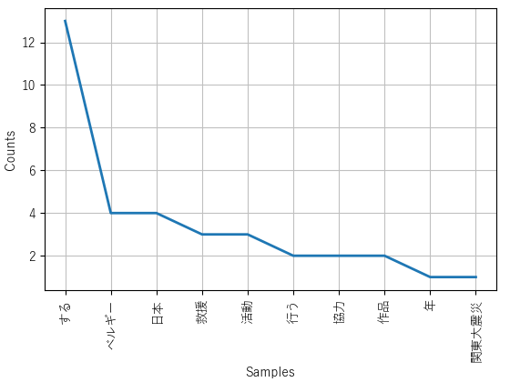Figure 1: Frequency distribution (filtered).

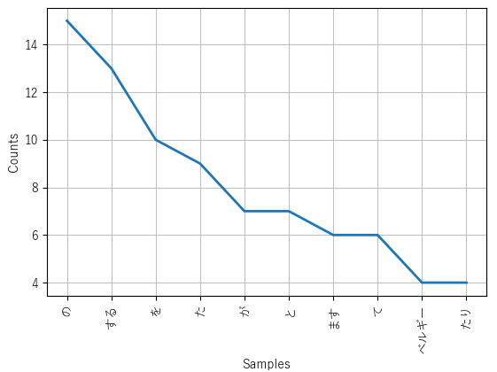Figure 2: Frequency distribution (unfiltered).

The script below takes several further steps to removing noise by filtering tokens based on their POS-tags (thus excluding particles, conjugations in the form of auxiliary verbs, pronouns, pre- and suffixes, symbols, exclamations, etc). Moreover, the script below uses, if available, the dictionary form of segmented words. Figure 2 is an illustration of the outcome when that step is not taken.

 1
 2
 3
 4
 5
 6
 7
 8
 9
10
11
12
13
14
15
16
17
18
19
20
21
22
23
24
25
26
27
28
29
30
31
32

# coding=utf-8

import MeCab
import neologdn
#Using tabs to separate lemmas and then tokenizing by splitting on tabs retains proper nouns separated by half-width spaces 
tagger = MeCab.Tagger("-F%m\\t --unk-feature 未知語")
from nltk.probability import FreqDist
from matplotlib import rcParams
rcParams['font.family'] = 'sans-serif'
rcParams['font.sans-serif'] = ['Hiragino Maru Gothic Pro', 'Yu Gothic', 'Meirio', 'Takao', 'IPAexGothic', 'IPAPGothic', 'VL PGothic', 'Noto Sans CJK JP']

CONTENT_WORD_POS = ("名詞", "動詞", "形容詞", "副詞", "未知語")
IGNORE = ("接尾", "非自立", "代名詞")

def is_content_word(feature):
    return feature.startswith(CONTENT_WORD_POS) and all(f not in IGNORE for f in feature.split(",")[:6])

if __name__ == '__main__':
    text = "１９２３年の関東大震災が起こった時、ベルギー人がためらわず、救援活動を行ったり資金集めをしたりしたのは、この友好的な日本との関係のためだと言えます。王族と、新たに設立されたベルギー国内委員会が協力して大規模な救援活動を実施しました。私の故郷アントワープを含むベルギーの全国各地でも教会と戦争の退役軍人が協力して「Japan Day」という催しを行いました。他にも、ベルギー人の芸術家達が作品を集めたり新作を発表したりして特別な貢献をしました。まずはブリュッセルで、次に日本で作品の展示発売や展覧会を開催し、売り上げや入場料の利益は全て救援活動のために寄付されました。日本の展覧会だけでも3万５千人もの観客が訪れたと報告されていて、その上、日本の皇太子様と皇后様が30点もの芸術品をご購入されたと聞いております。"
    text = neologdn.normalize(text, repeat=2)
    #some more noise removal
    text = ''.join([i for i in text if i.isalpha() or i.isspace()])
    result = tagger.parseToNode(text)

    content_words = []
    while result:
        if is_content_word(result.feature):
            lemma = result.feature.split(",")[6] if len(result.feature.split(",")) > 6 and result.feature.split(",")[6] is not "*" else result.surface
            content_words.append((lemma))
        result = result.next
    fdist = FreqDist(content_words)
    fdist.plot(10, cumulative=False)

Stop-words (optional)

Stop-words refers to the most commonly used words in natural language; words we might want to filter out of our corpora depending on the context. NLTK has stop-word functionality and comes with lists of stop-words for 16 different languages. Those do not include Japanese, however, and we will have to add that manually.

An NLTK stop-word list is merely a text-file of words separated by newlines and stored in nltk_data\corpora\stopwords by their language (without the .txt extension).⁴ For now I recommend this one (the same one we have used in the previous guide). Save this in the NLTK stopwords folder as ‘Japanese’, without .txt extension. figure 3 displays the result of running an edited python script filtering out stop-words.

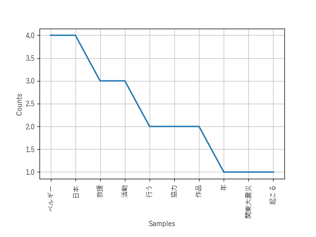Figure 3: Frequency distribution (filtered with stop-word list).

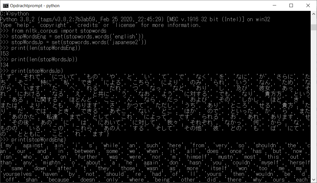Figure 4: Comparison of English and Japanese stop-word lists.

 1
 2
 3
 4
 5
 6
 7
 8
 9
10
11
12
13
14
15
16
17
18
19
20
21
22
23
24
25
26
27
28
29
30
31
32
33
34
35

# coding=utf-8

import MeCab
import neologdn
tagger = MeCab.Tagger("-F%m\\t --unk-feature 未知語")
from nltk.corpus import stopwords
from nltk.probability import FreqDist
from matplotlib import rcParams
rcParams['font.family'] = 'sans-serif'
rcParams['font.sans-serif'] = ['Hiragino Maru Gothic Pro', 'Yu Gothic', 'Meirio', 'Takao', 'IPAexGothic', 'IPAPGothic', 'VL PGothic', 'Noto Sans CJK JP']

CONTENT_WORD_POS = ("名詞", "動詞", "形容詞", "副詞", "未知語")
IGNORE = ("接尾", "非自立", "代名詞")

def is_content_word(feature):
    return feature.startswith(CONTENT_WORD_POS) and all(f not in IGNORE for f in feature.split(",")[:6])

if __name__ == '__main__':
    text = "１９２３年の関東大震災が起こった時、ベルギー人がためらわず、救援活動を行ったり資金集めをしたりしたのは、この友好的な日本との関係のためだと言えます。王族と、新たに設立されたベルギー国内委員会が協力して大規模な救援活動を実施しました。私の故郷アントワープを含むベルギーの全国各地でも教会と戦争の退役軍人が協力して「Japan Day」という催しを行いました。他にも、ベルギー人の芸術家達が作品を集めたり新作を発表したりして特別な貢献をしました。まずはブリュッセルで、次に日本で作品の展示発売や展覧会を開催し、売り上げや入場料の利益は全て救援活動のために寄付されました。日本の展覧会だけでも3万５千人もの観客が訪れたと報告されていて、その上、日本の皇太子様と皇后様が30点もの芸術品をご購入されたと聞いております。"
    text = neologdn.normalize(text, repeat=2)
    text = ''.join([i for i in text if i.isalpha() or i.isspace()])
    result = tagger.parseToNode(text)

    stop_words = stopwords.words('japanese')
    content_words = []

    while result:
        if is_content_word(result.feature):
            lemma = result.feature.split(",")[6] if len(result.feature.split(",")) > 6 and result.feature.split(",")[6] != "*" else result.surface
            if lemma not in stop_words:
                content_words.append((lemma))
        result = result.next

    fdist = FreqDist(content_words)
    fdist.plot(10, cumulative=False)

Sentiment analysis

[Coming soon: Sentiment analysis]

Bringing it all together: processing tweets

[Let’s apply this on a real-world example]

Wait! There is more!

The next guide in this series will expand on the methods outlined in the second guide, paying particular attention to the most common actors related to a certain keyword as well as their network.

• A Quick Guide to Data-mining & (Textual) Analysis of (Japanese) Twitter Part 1: Twitter Data Collection
• A Quick Guide to Data-mining & (Textual) Analysis of (Japanese) Twitter Part 2: Basic Metrics & Graphs
• A Quick Guide to Data-mining & (Textual) Analysis of (Japanese) Twitter Part 3: Natural Language Processing With MeCab, Neologd and KH Coder
• A Quick Guide to Data-mining & (Textual) Analysis of (Japanese) Twitter Part 5: Advanced Metrics & Graphs

On a final note, it is my aim to write tutorials like these in such a way that they provide enough detail and (technical) information on the applied methodology to be useful in extended contexts, while still being accessible to less IT-savvy students. If anything is unclear, however, please do not hesitate to leave questions in the comment section below.